Last summer, my friend Eric and I wanted to embed a citation graph. However, the existing Python implementations of node2vec are quite slow. I coded a faster version using numba which was good enough.
Can we make it even faster using mathematics?
The current version of the code works really well and is available on github.
Reminder about node2vec
node2vec is a famous technique to embed nodes of any (un)directed, (un)weighted network by stating a node should have an embedding reflecting its neighborhood.
It applies another famous technique from the field of natural language processing, the skip-gram model. Using this technique to produce word vectors is now referred to as word2vec.
From the node2vec paper:
Given the linear nature of text, the notion of a neighborhood can be naturally defined using a sliding window over consecutive words. Networks, however, are not linear, and thus a richer notion of a neighborhood is needed. To resolve this issue, we propose a randomized procedure that samples many different neighborhoods of a given source node.
To implement node2vec, one simply has to generate neighborhoods and plug them into an implementation of skip-gram word2vec, the most popular being gensim.
Biased walks
node2vec defines neighborhoods as biased random walks. Starting from a node, one produces a random walk by repeatedly sampling a neighbor of the last visited node.
The walk is biased using two parameters $p$ and $q$.
Supposing we just traversed the edge $(t, v)$, and are taking a decision in $v$, we assign a transition probability to $(v, x)$ that is proportional to $w_{vx} \cdot \alpha(t, x)$. $w_{vx}$ is the weight of this edge and
\[\alpha(t, x) = \begin{cases} \frac1p & \text{if } t = x \\ 1 & \text{if } dist(x, t) = 1 \\ \frac1q & \text{if } dist(x, t) = 2 \end{cases}\]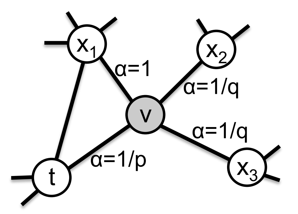
The problem of the above approach is that the transition probabilities depend on the two last visited nodes. The authors suggest to store them for every such pair first, which approximately multiplies the space complexity by the average degree $\bar d$. If you do, you can sample in $\mathcal{O}(1)$ (using the Alias method), else you can compute the probabilities on the fly in $\mathcal{O}(\bar d)$ (by merging sorted adjacency lists). Thus, if you only do one pass, there is a clear space advantage to do the computation on the fly!
In some cases, the sampling can be much faster: if the graph is unweighted and $p=q=1$, one can just sample any neighbor in $\mathcal{O}(1)$. Isn’t it surprising that changing these parameters a little bit messes up the whole complexity?
Rejection sampling
Let’s consider a simpler problem with an urn containing $b$ blue balls and $r$ red balls.
If we sample one ball uniformly, the probability to get a blue one is $\frac{b}{b+r}$.
Now suppose we want to multiply the weight of blue balls by 2, that is get a blue ball with probablity $\frac{2 b}{2 b+r}$. One solution would be to add $b$ blue balls. If $r$ is even, we could also halve it as $\frac{2 b}{2 b+r} = \frac{b}{b+\frac{r}{2}}$.
If we cannot remove half of the red balls, we could still paint half of them in white. When we draw a white ball, we can ignore it.
Instead of painting half of the red balls in white, we could also paint one half of each red balls in white. When drawing a mixed color ball, we can randomly select one of its colors and suppose the whole ball has this color. This is the idea of rejection sampling.

The formal definition of rejection sampling is that given a discrete probability distribution $\Pr[X = i] = p_i$ and weights $0 \le w_i \le 1$, one can sample from the distribution $\Pr[X = i] = \frac{p_i \cdot w_i}{Z}$ for some normalization constant $Z$.
The figure below summarizes the method:
- draw a point uniformly in the square
- if you are in the red zone, try again
- if you are in the green zone, return the index of the green bar

The downside of this method is that you might have to try multiple times if the red zone is too big.
If you want to know more about related techniques to sample discrete random variables (like the alias method), I recommend you to read this awesome essay: Darts, Dice, and Coins: Sampling from a Discrete Distribution.
Back to our problem
In our case, we have nodes with different weights, but it is costly to compute or store all of them, hence we are going to apply rejection sampling.
Changing our notations, the original probability distribution is (up to a constant)
\[\Pr(v \rightarrow x | t \rightarrow x) \sim w_{vx}\]and we want to transform it into
\[\Pr(v \rightarrow x | t \rightarrow x) \sim w_{vx} \cdot \alpha(t, x)\]In the figure above, $p$ corresponds to normalized $w_{vx}$ and $w$ is $\alpha(t, x)$.
Hence, the algorithm is simply:
- Choose a neighbor $x$ according to the graph weights, $w_{vx}$
- Determine $\alpha(t, x)$ by testing whether $x$ is $t$ or a neighbor of $t$
- Draw a Boolean variable with probability $\sim \alpha(t, x)$. If it is true, return $x$, else go back to step 1.
What is the complexity?
Step 1 costs $\mathcal{O}(1)$ with the alias method (see the essay above), or $\mathcal{O}(\log \bar d)$ with binary search and no additional memory.
Step 2 costs $\mathcal{O}(\log \bar d)$ using binary search on sorted adjacency lists. Constant time is possible with hash tables but with a greater (constant) memory usage.
How many times are they repeated? In other terms, how big is the red area?
The possible values of $\alpha(t, x)$ are $1$, $\frac1p$ and $\frac1q$. In general, $p < 1 < q$ and we have to normalize our values so that the largest is $1$. Hence, they become $\frac{p}{q}$, $p$ and $1$. The area of the green area is thus at least $\frac{p}{q}$. This is the weight of the previous node, so it only applies to one case. In practice, the area of the green area will be between $p$ and $1$ (going to nodes at distance 1 or 2 from the previous node). For the typical values reported in the paper, $p$ is between $\frac14$ and $1$.
The average complexity of this algorithm is thus $\mathcal{O}\left(\frac{\log \bar d}{p}\right) < \mathcal{O}(4 \cdot \log \bar d)$. In theory, one could get rid of the asymptotic $\log \bar d$ factor but at the cost of a larger constant factor.
Implementation details
Below is the full code to generate one walk and accelerate the code with numba.
The only abstractions I made for the sake of clarity are random_neighbor that samples a random neighbor according to the graph weights and is_neighbor that tests whether two nodes share an edge.
import numpy as np
from numba import njit


@njit(nogil=True)
def random_walk(walk_length, p, q, t):
    """sample a random walk starting from t
    """
    # Normalize the weights to compute rejection probabilities
    max_prob = max(1 / p, 1, 1 / q)
    prob_0 = 1 / p / max_prob
    prob_1 = 1 / max_prob
    prob_2 = 1 / q / max_prob

    # Initialize the walk
    walk = np.empty(walk_length, dtype=indices.dtype)
    walk[0] = t
    walk[1] = random_neighbor(t)

    for j in range(2, walk_length):
        while True:
            new_node = random_neighbor(walk[j - 1])
            r = np.random.rand()
            if new_node == walk[j - 2]:
                # back to the previous node
                if r < prob_0:
                    break
            elif is_neighbor(walk[j - 2], new_node):
                # distance 1
                if r < prob_1:
                    break
            elif r < prob_2:
                # distance 2
                break
        walk[j] = new_node

    return walk
Conclusion
Using rejection sampling, one can implement biased random walks for node2vec in logarithmic (or even constant) instead of linear time without additional memory or precomputation.
This improvement is a bit overkill in practice: the average degree $\bar d$ typically ranges between 20 and 100. The naive implementation (which computes all transition probabilities at every step) already runs much faster than gensim’s word2vec when implemented in numba, but rejection sampling makes it even faster.
It was fun anyway to find an application of randomized algorithms in machine learning!
Other nice features of fastnode2vec are distributing the random walk generation accross gensim threads and providing a CLI. I recommend you to try it!