A common problem we have at Tiime and in many other places is to adjust the rate limit of a service to the load. This is how we do it.

Rate limiting

Rate limiting typically controls the number of requests per unit of time a service can handle. When the rate limit is reached, the service refuses new requests until the time unit is over. We can also decide to wait until the time unit is over before serving a new request.

There are many other implementations of rate limiting on Github but I couldn’t find any that were exactly what I wanted so I implemented my own there.

Modelling the problem

We assume that the calls arrive according to a Poisson process, which is the simplest model for a random arrival process. The Poisson process is characterized by a rate parameter $\mu$ which is the average number of events per unit of time. We define this unit of time as the rate limit period. We want to compute the probability of the service to respect the rate limit over a given duration. In a typical case, the rate limit period is one minute and the duration is one hour, which we can express as 60 units of time.

Typically, we compute the Poisson rate $\mu$ by counting how many requests we got during the hour of the week with the heaviest load and want to make sure that the probability of exceeding our rate limit over a given duration (e.g. one hour) is low enough.

To simulate the Poisson process over this duration, we can use the following code:

import numpy as np
from numba import njit

@njit
def poisson_process(mu: float, duration: float) -> np.ndarray:
    """Simulate a Poisson process with rate `mu` over `duration`."""
    n_events = np.random.poisson(mu * duration)
    if n_events == 0:
        return np.empty(0)
    events = np.random.uniform(low=0, high=duration, size=n_events)
    events.sort()
    return events

poisson_process(0.5, 5.0)
# array([1.18687599, 3.77746169])

Given an array of event times, we want to check that the rate limit is respected. In other terms, if the events are $e_i$, we want to check that all intervals of size 1 contain less than rate_limit events: $\forall x, \#\{i \mid x \leq e_i \leq x + 1\} \leq \text{rate_limit}$

or equivalently that there is no sequence of rate_limit events that are contained in a window of size 1: $\forall i, e_{i + \text{rate_limit}} - e_{i} \geq 1$

@njit
def success(events: np.ndarray, rate_limit: int) -> bool:
    for i in range(rate_limit, len(events)):
        if events[i] - events[i - rate_limit] < 1.0:
            return False
    return True

success([0.1, 0.3], 2)
# True
success([0.1, 0.3, 1.0], 2)
# False

By the power of numeric simulation, we can compute the probability of success by averaging over many simulations.

from numba import prange


@njit(parallel=True)
def success_prob_sim(mu, duration, rate_limit, n_samples=100_000):
    total = 0
    for _ in prange(n_samples):
        poisson = poisson_process(mu, duration)
        if success(poisson, rate_limit):
            total += 1
    return total / n_samples


success_prob_sim(0.5, 5.0, 2)
# 0.86141

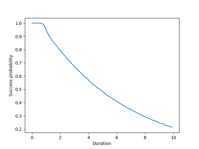
In fact, we can even plot the success probability as a function of the duration:

import matplotlib.pyplot as plt

durations = np.arange(0, 10, 0.1)
simulated = [success_prob_sim(mu=10.0, duration=d, rate_limit=15) for d in durations]
plt.plot(durations, simulated)
plt.xlabel("Duration")
plt.ylabel("Success probability")
plt.show()

As expected, the success probability decreases from $1$ to $0$ as the duration increases from $0$ to $\infty$. When duration is $0$, the probability is $1$ because there is no event, and the longer you wait, the more likely you are to exceed the rate limit. Eventually, if you wait long enough, you will always exceed the rate limit.

It also seems to closely follow a power law when the duration is large enough.

How to compute it faster?

success_prob_sim is nice but still quite costly to compute, plus it is not guaranteed to be monotonic, which makes it difficult to use binary search in practice.

Thanks to the help of Martin Ridout (who already helped me with another problem), I was able to relate this problem to the concept of scan statistic.

Unfortunately, there is no known efficient general closed-form expression for the success probability we are looking for.

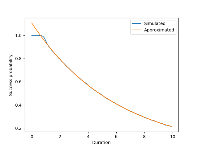
However, I found this paper from 1982: Approximations for distributions of scan statistics which provides a good enough solution. In this paper, Naus considers the exact same problem and, noting like me that the curve above is very well approximated by a power law, proposes to use the following formula:

where $f(d)$ is the success probability for duration $d$.

It also provides simple exact expressions for $f(2)$ and $f(3)$ (see Theorem 1 in the paper).

Thanks to this, we can now compute the success probability for any duration in constant time. You can find the full implementation here.

from malib import RateLimiter

rl = RateLimiter(max_calls=15, period=1.0)
approximated = [1 - rl.prob_exceeded_poisson(mu=10.0, duration=d) for d in durations]
plt.plot(durations, simulated, label="Simulated")
plt.plot(durations, approximated, label="Approximated")
plt.xlabel("Duration")
plt.ylabel("Success probability")
plt.legend()
plt.show()