Let’s start with a brain teaser. We consider 3 Gaussian random variables $\mathcal{N}(\mu, \sigma)$ defined by their mean and standard deviation: $A\sim\mathcal{N}(0, 1)$, $B\sim\mathcal{N}(0, 10)$ and $C\sim\mathcal{N}(1, 1)$. You have to bet on which variable has the highest value. What would you bet on?
What intuition tells us
If you followed your probability and statistics classes, you probably bet on $C$, right? After all, it has the highest mean, so it should yield the highest value most of the time.
Let us draw the probability distribution functions of those 3 variables:
import numpy as np
from scipy.stats import norm
import matplotlib.pyplot as plt

plt.rc('axes', linewidth=2)
plt.axhline(linewidth=1, color='k')
plt.axvline(linewidth=1, color='k')
plt.xlim(-10, 10)
plt.ylim(-.4, .8)
plt.grid(True, which='both')

x = np.linspace(-10, 10, 1000)
A = norm(0, 1)
B = norm(0, 10)
C = norm(1, 1)
plt.plot(x, A.pdf(x), label='A')
plt.plot(x, B.pdf(x), label='B')
plt.plot(x, C.pdf(x), label='C')

plt.legend()
plt.show()
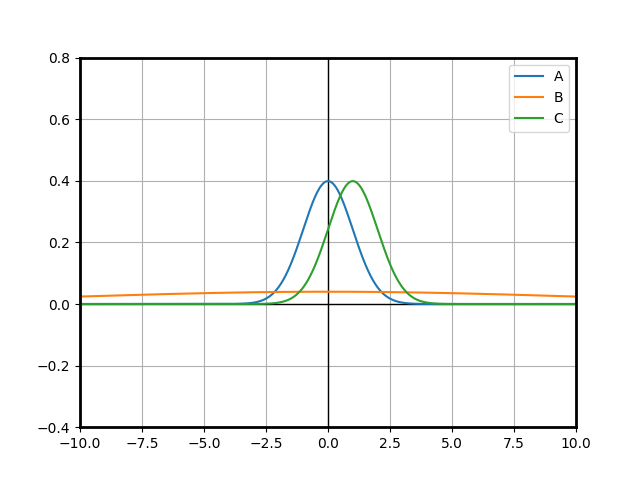
First, it looks straightforward that there is no chance that $A$ can be a good choice: suppose we had 2 $A$’s, then no one has more chances to win than the other by symmetry. Now add $1$ to all the outcomes of one of the variables and it is obvious that that variable just gained a massive advantage over the other one.
What about $B\sim\mathcal{N}(0, 10)$ and $C\sim\mathcal{N}(1, 1)$? At first glance, most people will say that $C$ should win more: it has a higher mean. Indeed, let’s suppose that $C$ is centered with mean $0$ and thus follows the same law as $A$. We can show that for each situation where $B$ wins against $C$, there is a situation with the same probability where $C$ wins against $B$: just flip the signs of $B$ and $C$. Since both distributions are symmetric, the probability of $B$ winning is the same as the probability of this nerfed $C$ winning. Thus, it is obvious that the real $C$ has a higher chance of winning than the real $B$.
This problem is fun because there are a lot of real-life situations where you can apply a similar model. Those situations involve a decision where you have multiple choices, some which are more risky than the others, and you have to pick the best one.
For example, it is common for highly competitive sectors to use venture capital money to keep prices low and gain adoption, until they have a sufficient market share and can become profitable. An investor will have to choose between a few startups to invest in (if they don’t invest in all of them). Some startups have advantages that convert into a better expectation of results with a lower deviation, like experienced founders or partnerships with established market players. Other startups will on the opposite try a risky strategy that could pay off, like a new technology or an original go-to-market approach. The investor will have to choose which startup to invest in to maximize the probability of that startup succeeding the most.
Where intuition fails
Let’s do some simulations to see what happens:
>>> np.bincount(np.argmax([A.rvs(10000), B.rvs(10000), C.rvs(10000)], 0))
array([1336, 4579, 4085])
Ouch! There goes our intuition. The variable with the highest mean does not have the highest probability of winning. Why is that?
To confirm, let’s confirm what happens when comparing only $B$ and $C$:
>>> np.bincount(np.argmax([B.rvs(10000), C.rvs(10000)], 0))
array([4540, 5460])
What about adding other instances of A?
>>> np.bincount(np.argmax([A.rvs(10000), A.rvs(10000), B.rvs(10000), C.rvs(10000)], 0))
array([ 974,  990, 4515, 3521])
>>> np.bincount(np.argmax([A.rvs(10000), A.rvs(10000), A.rvs(10000), B.rvs(10000), C.rvs(10000)], 0))
array([ 777,  816,  790, 4444, 3173])
Interesting! The more instances of $A$ we add, the more the probability of $C$ winning decreases, but the probability of $B$ winning stays about the same. The “leftovers” are distributed between the instances of $A$.
A simple explanation
$A$ and $B$ are focused on the same region around $0$ and $1$ respectively. Thus, they are “competing” for the same space. This is obvious as we add more instances of $A$.
On the other side, $C$ is focused on a different region. Of course, it has a lot of chances to be negative. But when it is positive, it is much more likely to be higher than $B$. And when it wins against $B$, it is very unlikely to lose against $A$, even when there are a lot of $A$’s.
A more formal approach
We can even compute the actual probabilities that each variable wins.
As a vector, the 3 variables form a multinomial distribution. Finding out a probability is the same as integrating the probability density function of that multinomial distribution. However, it is quite hard to express the region of the space $\{A > B\} \cap \{A > C \}$.
Instead, we are going to use a trick: what if we substracted $A$ from the two other variables? Now we are trying to integrate over $\{B - A < 0\} \cap \{C - A < 0\}$. If we can express the joint law of $B-A$ and $C-A$, then we reduced the problem to a 2-dimensional integral.
It is a well known fact that (with a slight abuse of notation) $\mathcal{N}(\mu_1, \sigma_1) + \mathcal{N}(\mu_2, \sigma_2) \sim \mathcal{N}\left(\mu_1 + \mu_2, \sqrt{\sigma_1^2 + \sigma_2^2}\right)$. Obviously, the substraction works the same way by substracting the means: $\mathcal{N}(\mu_1, \sigma_1) - \mathcal{N}(\mu_2, \sigma_2) \sim \mathcal{N}\left(\mu_1 - \mu_2, \sqrt{\sigma_1^2 + \sigma_2^2}\right)$
Now, there is an even more amazing fact, which is that multinomial variables are actually stable under linear transformations. This implies that $\begin{pmatrix} B-A \\ C-A \end{pmatrix}$ follows a multinomial law.
Thus, we can completely describe the distribution of $\begin{pmatrix} B-A \\ C-A \end{pmatrix}$ by the mean vector and the covariance matrix.
The mean is trivial to compute: $\begin{pmatrix} \mu_B - \mu_A \\ \mu_C - \mu_A \end{pmatrix}$.
The covariance is not much more complicated: we have already computed the standard deviation of each variable, so we just need to compute the covariance between $B-A$ and $C-A$. This is very easy, as $B$ and $C$ are still independant, hence the covariance is just the variance of $A$. We get:
$\begin{pmatrix} B-A \\ C-A \end{pmatrix} \sim \mathcal{N}\left(\begin{pmatrix} \mu_B - \mu_A \\ \mu_C - \mu_A \end{pmatrix}, \begin{pmatrix} \sqrt{\sigma_A^2 + \sigma_B^2} & \sigma_A \\ \sigma_A & \sqrt{\sigma_A^2 + \sigma_B^2} \end{pmatrix}\right) = \mathcal{N}\left(\begin{pmatrix} 0 \\ 1 \end{pmatrix}, \begin{pmatrix} \sqrt{101} & 1 \\ 1 & \sqrt{2} \end{pmatrix}\right)$
We can now compute the probability of $A$ winning using the scipy.stats.multivariate_normal.cdf function. Behind the scenes, it uses a Monte-Carlo method on a reparametrization to compute the integral following this paper.
import numpy as np
from scipy.stats import multivariate_normal


def remove(arr, idx):
    return np.concatenate((arr[:idx], arr[idx + 1 :]))


def prob(mean, std):
    n = len(mean)
    return [
        multivariate_normal.cdf(
            [0] * (n - 1),
            mean=remove(mean, idx) - mean[idx],
            cov=np.full((n - 1, n - 1), std[idx] ** 2) + np.diag(remove(std, idx) ** 2),
        )
        for idx in range(n)
    ]


print(prob([0, 0, 1], [1, 10, 1]))
The program gives [0.1285997208467189, 0.4524428550415489, 0.4189574241117322] which is very close to the empirical results we got before, hence $B$ will win more than 45% of the time and $C$ only 42%. You can play with the parameters to see how the probabilities change. For example, prob([0, 1], [10, 1]) tells us that in a context between only $B$ and $C$, $C$ would win 54% of the time.
Conclusion
I think this is a very interesting result. It shows that the probability of a variable having the highest value is not just a matter of the individual variables that it will be compared against but of all the system.
When multiple entities are competing for the same space, their chances of winning decrease linearly. On the other hand, they actually increase the chances of those who are taking riskier bets because they are not in the same fight.